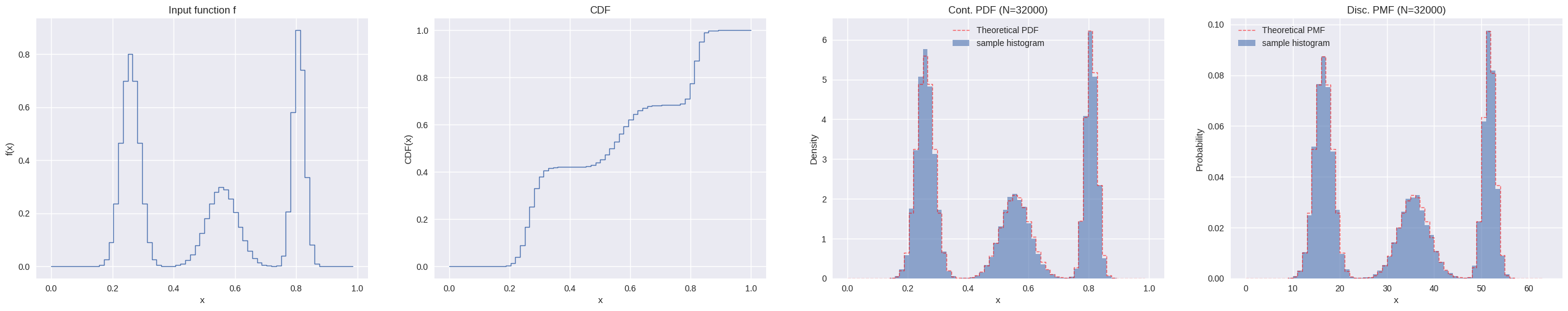
区分的定数分布とは,定義域を複数の区分(区間,セル,ビンなど)に分割し,それぞれの区分内で確率密度関数が一定値を取るように定義された確率分布である.
コード
import gcimport numpy as npimport matplotlib.pyplot as pltimport matplotlib.gridspec as gridspec# from mpl_toolkits.axes_grid1 import make_axes_locatable import numpy.typing as nptfrom typing import TypeAlias, overload# from typing import overload = np.random.default_rng(12345 )# print(plt.style.available) "seaborn-v0_8" )
1次元の区分的定数分布
区間 \([0,1]\) を \(\Delta=\frac{1}{N}\) で分割し,端点 \(x_{i}=i\Delta\quad(i=0,\dots,N)\) とする.
\[
f(x)=
\begin{cases}
v_{0} \quad x_{0}\le x\lt x_{1}\\
v_{1} \quad x_{1}\le x\lt x_{2}\\
\vdots\\
v_{N-1} \quad x_{N-1}\le x\lt x_{N}\\
\end{cases}
\]
積分は,
\[
c
=\int_{0}^{1} f(x)\,dx
=\sum_{i=0}^{N-1} \int_{x_{i}}^{x_{i+1}} f(x)\,dx
=\sum_{i=0}^{N-1}v_{i}\Delta
=\sum_{i=0}^{N-1}\frac{v_{i}}{N}
\]
確率密度関数は,
\[
p(x)=\frac{f(x)}{c}
\]
累積分布関数は区分的に線形な関数となり,その値は各点 \(x_{i}\) において次のように定義される.
\[
\begin{align*}
P(x_{0})&=0\\
P(x_{i})
&=\int_{x_{0}}^{x_{i}} p(x)\,dx
=\int_{x_{0}}^{x_{i-1}} p(x)\,dx+\int_{x_{i-1}}^{x_{i}} p(x)\,dx\\
&=P(x_{i-1})+\frac{v_{i-1}}{cN}
,\quad(i=1,\dots,N)
\end{align*}
\]
\([x_{i},x_{i+1})\) では,累積分布関数は傾き \(v_{i}/c\) で線形に増加する.累積分布関数は単調増加なので,任意の \(\zeta\) に対し \(x\) の値は必ず \([x_{i},x_{i+1})\) に存在し,
\[
P(x_{i})\le\zeta\lt P(x_{i+1})
\]
が成り立つ.累積分布関数の値の配列が与えられていれば,このような \(P(x_{i})\) の組は二分探索によって効率的に求めることができる.よって逆関数法によるサンプリングでは,対応する区間が決まれば \(x\) の値は次のように与えられる.
\[
x=\left(i+\frac{\zeta-P(x_{i})}{P(x_{i+1})-P(x_{i})}\right)\Delta
\]
コード
class Distribution1D:def __init__ (self , f: npt.NDArray[np.floating], * , dtype: npt.DTypeLike = np.float32) -> None :self .dtype = np.dtype(dtype)self .func = np.asarray(f, dtype= self .dtype)= len (self .func)# Compute integral of step function at x_i self .cdf = np.zeros(n + 1 , dtype= self .dtype)self .cdf[1 :] = np.cumsum(self .func / n, axis= 0 )# Transform step function integral into CDF self .func_int = self .cdf[n]if self .func_int == self .dtype.type (0 ):self .cdf = np.linspace(0 , 1 , n + 1 , dtype= self .dtype)else :self .cdf /= self .func_intdef count(self ) -> int :return len (self .func)@overload def sample_continuous(self , u: float | np.floating) -> tuple [np.floating, np.floating, np.int32]: ...@overload def sample_continuous(self , u: npt.NDArray[np.floating]) -> tuple [npt.NDArray[np.floating], npt.NDArray[np.floating], npt.NDArray[np.int32]]: ...def sample_continuous(self , u):= np.asarray(u, dtype= self .dtype)# Find surrounding CDF segments and offset = np.searchsorted(self .cdf, u, side= "right" ) - 1 = np.clip(offset, 0 , len (self .cdf) - 2 ).astype(np.int32)# Compute offset along CDF segment = u - self .cdf[offset]= self .cdf[offset + 1 ] - self .cdf[offset]= np.where(seg > self .dtype.type (0 ), du / seg, du)# Compute PDF for sampled offset = (offset.astype(self .dtype) + du) / self .count()= self .func[offset] / self .func_int# Return x in [0,1) corresponding to sample if np.ndim(u) == 0 :return x[()], pdf[()], offset[()]return x, pdf, offset@overload def sample_discrete(self , u: float | np.floating) -> tuple [np.int32, np.floating, np.floating]: ...@overload def sample_discrete(self , u: npt.NDArray[np.floating]) -> tuple [npt.NDArray[np.int32], npt.NDArray[np.floating], npt.NDArray[np.floating]]: ...def sample_discrete(self , u):= np.asarray(u, dtype= self .dtype)# Find surrounding CDF segments and offset = np.searchsorted(self .cdf, u, side= "right" ) - 1 = np.clip(offset, 0 , len (self .cdf) - 2 ).astype(np.int32)= self .func[offset] / (self .func_int * self .count())= (u - self .cdf[offset]) / (self .cdf[offset + 1 ] - self .cdf[offset])if np.ndim(u) == 0 :return offset[()], pdf[()], u_remapped[()]return offset, pdf, u_remapped@overload def discrete_pdf(self , index: int | np.integer) -> np.floating: ...@overload def discrete_pdf(self , index: npt.NDArray[np.integer]) -> npt.NDArray[np.floating]: ...def discrete_pdf(self , index):return self .func[index] / (self .func_int * self .count())
コード
def histogram_1d(sampler, sample_size, batch_size, rng, bins, range = None ):= sampler(1 , rng).dtypeif isinstance (bins, int ):= np.linspace(* range , bins + 1 , dtype= dtype)else := np.asarray(bins, dtype= dtype)= np.zeros(len (edges) - 1 , dtype= np.int64)= sample_sizewhile remaining > 0 := min (batch_size, remaining)= sampler(current_batch, rng)= np.histogram(samples, bins= edges, range = range , density= False )+= H_batch-= current_batchdel samples, H_batch= H_total / (sample_size * np.diff(edges))return H_density, edgesdef plot_distribution_1d(distr: Distribution1D, sample_size: int , rng: np.random.Generator) -> None := distr.count()= np.linspace(0 , 1 , n + 1 , dtype= distr.dtype)= np.arange(distr.count())def continuous_sampler(sample_size: int , rng: np.random.Generator):return distr.sample_continuous(rng.random(sample_size, dtype= distr.dtype))[0 ]def discrete_sampler(sample_size: int , rng: np.random.Generator):return distr.sample_discrete(rng.random(sample_size, dtype= distr.dtype))[0 ]= ["title" : "Input function f" , "ylabel" : "f(x)" , "plot_fn" : lambda ax: ax.step(x[:- 1 ], distr.func, where= "post" , linewidth= 1 )},"title" : "CDF" , "ylabel" : "CDF(x)" , "plot_fn" : lambda ax: ax.step(x, distr.cdf, where= "post" , linewidth= 1 )},"title" : f"Cont. PDF (N= { sample_size} )" ,"ylabel" : "Density" ,"legend" : True ,"data_fn" : lambda : (100000 , rng, bins= x),/ distr.func_int,"plot_fn" : lambda ax, hist_data, pdf: (1 ][:- 1 ], hist_data[0 ], width= np.diff(hist_data[1 ]), align= "edge" , alpha= 0.6 , label= "sample histogram" ),1 ][:- 1 ], pdf, where= "post" , color= "red" , linestyle= "--" , linewidth= 1 , alpha= 0.6 , label= "Theoretical PDF" ),"title" : f"Disc. PMF (N= { sample_size} )" ,"ylabel" : "Probability" ,"legend" : True ,"data_fn" : lambda : (100000 , rng, bins= np.arange(distr.count() + 1 )),"plot_fn" : lambda ax, hist_data, pdf: (1 ][:- 1 ], hist_data[0 ], width= np.diff(hist_data[1 ]), align= "edge" , alpha= 0.6 , label= "sample histogram" ),1 ][:- 1 ], pdf, where= "post" , color= "red" , linestyle= "--" , linewidth= 1 , alpha= 0.6 , label= "Theoretical PMF" ),= (1 , len (data))= plt.rcParams.get("figure.figsize" )= (base_w * nrows_ncols[1 ], base_h * nrows_ncols[0 ])= {"xlabel" : "x" }= plt.subplots(nrows= nrows_ncols[0 ], ncols= nrows_ncols[1 ], subplot_kw= subplot_kw, figsize= figsize)= np.atleast_1d(axs).flatten()for ax, datum in zip (axs, data):= ()if "data_fn" in datum:= datum["data_fn" ]() # type: ignore "plot_fn" ](ax, * res) # type: ignore "title" ])"ylabel" ])True )if datum.get("legend" ):
コード
def gaussian1d(x, x0, sigma):return np.exp(- ((x - x0) ** 2 ) / (2 * sigma** 2 ))= np.linspace(0 , 1 , 64 + 1 )= [(0.25 , 0.03 , 0.8 ), (0.55 , 0.05 , 0.3 ), (0.8 , 0.02 , 0.9 )]= sum (a * gaussian1d(x, x0, s) for x0, s, a in peaks_1d)= f[:- 1 ].astype(np.float32)500 * f.size, rng)
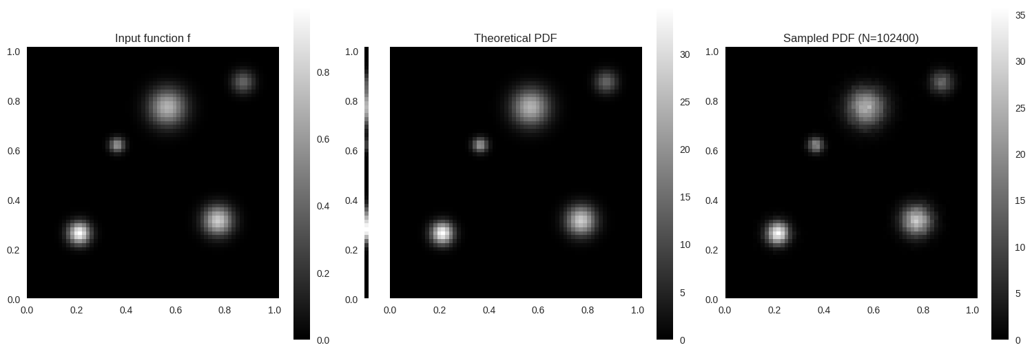
2次元の区分的定数分布
2次元関数 \(f(u,v)\) が,\(u_{i}\in[0,1,\dots,n_{u}-1],\,v_{j}\in[0,1,\dots,n_{v}-1]\) に対して \(f[u_{i},v_{j}]\) の値によって定義され,\(f[u_{i},v_{j}]\) は範囲 \([\frac{i}{n_{u}},\frac{i+1}{n_{u}})\times[\frac{j}{n_{v}},\frac{j+1}{n_{v}})\) で一定の値を取るとする.連続値 \((u,v)\) が与えられたとき,対応する離散インデクス \((\tilde{u},\tilde{v})\) を \(\tilde{u}=\lfloor n_{u}u\rfloor,\,\tilde{v}=\lfloor n_{v}v\rfloor\) と定義し,\(f(u,v)=f[\tilde{u},\tilde{v}]\) とする.
\(f\) の積分は \(f[u_{i},v_{j}]\) の値の単純な和になる.
\[
I_{f}
=\iint_{[0,1]^{2}} f(u,v)\,dudv
=\sum_{i=0}^{n_{u}-1}\sum_{j=0}^{n_{v}-1}\int_{\frac{i}{n_{u}}}^{\frac{i+1}{n_{u}}}\int_{\frac{j}{n_{v}}}^{\frac{j+1}{n_{v}}} f[u_{i},v_{j}]\,dvdu\\
=\frac{1}{n_{u}n_{v}}\sum_{i=0}^{n_{u}-1}\sum_{j=0}^{n_{v}-1} f[u_{i},v_{j}]
\]
\(f\) の同時確率密度関数は,
\[
p(u,v)
=\frac{f(u,v)}{I_{f}}
=\frac{f[\tilde{u},\tilde{v}]}{\frac{1}{n_{u}n_{v}}\sum_{i=0}^{n_{u}-1}\sum_{j=0}^{n_{v}-1} f[u_{i},v_{j}]}
\]
周辺確率密度関数は,\(f[u_{i},v_{j}]\) の値の和として計算できる.
\[
p(v)
=\int_{0}^{1} p(u,v)\,du
=\frac{1}{I_{f}}\int_{0}^{1} f(u,v)\,du
=\frac{\frac{1}{n_{u}}\sum_{i=0}^{n_{u}-1} f[u_{i},\tilde{v}]}{I_{f}}
\]
この関数は,\(\tilde{v}\) にのみ依存するため,\(n_{v}\) 個の値で定義される区分的定数1次元関数 \(p[\tilde{v}]\) となる.\(v\) のサンプルが与えられたとき,条件付き確率密度関数は,
\[
p(u|v)
=\frac{p(u,v)}{p(v)}
=\frac{\frac{f[\tilde{u},\tilde{v}]}{I_{f}}}{p[\tilde{v}]}
=\frac{f[\tilde{u},\tilde{v}]}{\frac{1}{n_{u}}\sum_{i=0}^{n_{u}-1} f[u_{i},\tilde{v}]}
\]
特定の \(\tilde{v}\) の値が与えられたとき,\(p[\tilde{u}|\tilde{v}]\) は \(\tilde{u}\) の区分的定数1次関数であり,通常の1次元手法でサンプリングが可能である.\(\tilde{v}\) の各値に対して \(n_{v}\) 個の異なる1次元条件付き密度が存在する.
コード
class Distribution1DBatch:def __init__ (self , funcs: npt.NDArray[np.floating], * , dtype: npt.DTypeLike = np.float32):# funcs: shape (M, N) (M distributions, each length N) self .dtype = np.dtype(dtype)self .func = np.asarray(funcs, dtype= self .dtype)= self .func.shape# Compute integral of step function at x_i self .cdf = np.zeros((M, N + 1 ), dtype= self .dtype)self .cdf[:, 1 :] = np.cumsum(self .func / N, axis= 1 )# Transform step function integral into CDF self .func_int = self .cdf[:, - 1 ].copy()= self .func_int == self .dtype.type (0 )self .cdf[mask] = np.linspace(0 , 1 , N + 1 , dtype= self .dtype)= ~ maskself .cdf[mask] /= self .func_int[mask, None ]def sample_continuous(self , u: npt.NDArray[np.floating], batch_idx: npt.NDArray[np.integer]) -> tuple [npt.NDArray[np.floating], npt.NDArray[np.floating], npt.NDArray[np.int32]]:= np.asarray(u, dtype= self .dtype)= batch_idx= self .cdf[rows]= self .func.shape# Find surrounding CDF segments and offset = (cdf_rows[:, 1 :] <= u[:, None ]).sum (axis= 1 ) # vectorized searchsorted = np.clip(cols, 0 , N - 1 , dtype= np.int32)# Compute offset along CDF segment = np.arange(len (u))= u - cdf_rows[row_idx, cols]= cdf_rows[row_idx, cols + 1 ] - cdf_rows[row_idx, cols]= np.where(seg > self .dtype.type (0 ), du / seg, du)# Return x in [0,1) corresponding to sample = (cols.astype(self .dtype) + du) / N= self .func[rows, cols] / self .func_int[rows]return x, pdf, colsclass Distribution2D:def __init__ (self , func: npt.NDArray[np.floating], * , dtype: npt.DTypeLike = np.float32) -> None :self .dtype = np.dtype(dtype)= func.shape# Compute conditional sampling distribution for v_tilde self .conditional_v = Distribution1DBatch(func, dtype= self .dtype)# Compute marginal sampling distribution p[v_tilde] = self .conditional_v.func_intself .marginal = Distribution1D(marginal_func, dtype= self .dtype)def sample_continuous(self , u):= np.asarray(u, dtype= self .dtype)= u.ndim == 1 = np.atleast_2d(u)= self .marginal.sample_continuous(u[:, 1 ])= self .conditional_v.sample_continuous(u[:, 0 ], v)= np.stack([d0, d1], axis=- 1 )= pdf0 * pdf1if is_single:return np.squeeze(x, axis= 0 ), np.squeeze(pdf, axis= 0 )[()]return x, pdfdef pdf(self , p):= np.asarray(p, dtype= self .dtype)= p.ndim == 1 = np.atleast_2d(p)= self .conditional_v.func.shape= np.clip((p[:, 0 ] * nu).astype(np.int32), 0 , nu - 1 )= np.clip((p[:, 1 ] * nv).astype(np.int32), 0 , nv - 1 )= self .conditional_v.func[iv, iu] / self .marginal.func_intif is_single:return np.squeeze(pdf, axis= 0 )[()]return pdf
コード
def histogram_2d(sampler, sample_size, batch_size, rng, bins, range = None ):= sampler(1 , rng).dtypeif isinstance (bins, int ):= np.linspace(* range , bins + 1 , dtype= dtype)= np.linspace(* range , bins + 1 , dtype= dtype)elif isinstance (bins[0 ], int ) and isinstance (bins[1 ], int ):= np.linspace(* range [0 ], bins[0 ] + 1 , dtype= dtype)= np.linspace(* range [1 ], bins[1 ] + 1 , dtype= dtype)else := np.asarray(bins[0 ])= np.asarray(bins[1 ])= np.zeros((len (xedges) - 1 , len (yedges) - 1 ))= sample_sizewhile remaining > 0 := min (batch_size, remaining)= sampler(current_batch, rng)= np.histogram2d(samples[:, 0 ], samples[:, 1 ], bins= (xedges, yedges), range = range , density= False )+= H_batch-= current_batchdel samples, H_batch= np.diff(xedges)[:, None ] * np.diff(yedges)[None , :]= H_total / (sample_size * area)return H_density, xedges, yedgesdef plot_distribution_2d(distr: Distribution2D, sample_size: int , rng: np.random.Generator) -> None :def gen_marginal_pdf():= np.arange(distr.marginal.count())= distr.marginal.func[indices] / distr.marginal.func_intreturn pdf[:, None ]def gen_pdf():= distr.conditional_v.func.shape= np.linspace(0 , 1 , nu + 1 , dtype= distr.dtype)[:- 1 ]= np.linspace(0 , 1 , nv + 1 , dtype= distr.dtype)[:- 1 ]= np.meshgrid(u, v)= np.stack([U.ravel(), V.ravel()], axis=- 1 )return distr.pdf(points).reshape(nv, nu)def gen_histogram():= lambda sample_size, rng: distr.sample_continuous(rng.random((sample_size, 2 ), dtype= distr.dtype))[0 ]= histogram_2d(sampler, sample_size, 100000 , rng, bins= (nu, nv), range = ((0 , 1 ), (0 , 1 )))return H.T= distr.conditional_v.func.shape= ["title" : "Input function f" , "data_fn" : lambda : distr.conditional_v.func, "width" : nu},"title" : "" , "hide_cbar" : True , "hide_xticks" : True , "data_fn" : gen_marginal_pdf, "width" : 1 },"title" : "Theoretical PDF" , "hide_yticks" : True , "sharey_with" : 1 , "data_fn" : gen_pdf, "width" : nu},"title" : f"Sampled PDF (N= { sample_size} )" , "data_fn" : gen_histogram, "width" : nu},= nv / nu= 5 = subplot_width * aspect_ratio= (subplot_width * (len (data) - 1 ), subplot_height)= plt.figure(figsize= figsize, constrained_layout= True )= 0.1 )= gridspec.GridSpec(1 , len (data), figure= fig, width_ratios= [datum["width" ] for datum in data])= [fig.add_subplot(gs[i]) for i in range (len (data))]= np.linspace(0 , nu - 1 , 6 )= [f" { x:.1f} " for x in np.linspace(0 , 1 , 6 )]= np.linspace(0 , nv - 1 , 6 )= [f" { y:.1f} " for y in np.linspace(0 , 1 , 6 )]for ax, datum in zip (axs, data):= datum["data_fn" ]() # type: ignore = X.shape= ax.imshow(X, cmap= "gray" , aspect= "equal" , interpolation= "nearest" , extent= [0 , nx, 0 , ny])"title" ])0 , nx)0 , ny)False )if datum.get("hide_xticks" ):= "x" , which= "both" , bottom= False , labelbottom= False )if datum.get("hide_yticks" ):= "y" , which= "both" , left= False , labelleft= False )if "sharey_with" in datum:"sharey_with" ]])= fig.colorbar(im, ax= ax)not datum.get("hide_cbar" , False ))
コード
def gaussian2d(x, y, x0, y0, sigma):return np.exp(- ((x - x0) ** 2 + (y - y0) ** 2 ) / (2 * sigma** 2 ))= 64 , 64 = np.linspace(0 , 1 , nu + 1 )[:- 1 ]= np.linspace(0 , 1 , nv + 1 )[:- 1 ]= np.meshgrid(u_edges, v_edges)= [0.20 , 0.25 , 0.03 , 1.0 ),0.75 , 0.30 , 0.04 , 0.8 ),0.55 , 0.75 , 0.05 , 0.7 ),0.35 , 0.60 , 0.02 , 0.6 ),0.85 , 0.85 , 0.03 , 0.4 ),= sum (a * gaussian2d(U, V, u0, v0, s) for u0, v0, s, a in peaks_2d)= f[::- 1 ]= f.astype(np.float32)25 * f.size, rng)
使用例
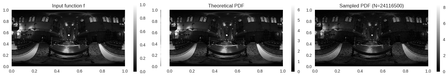
球面上の方向 \(\omega\) を選ぶ確率は,その方向の輝度 \(L(\omega)\) に比例すると考えられる.微小な立体角要素 \(d\omega\) を用いると,
\[
p_{\Omega}(\omega)\,d\omega
\propto L(\omega)\,d\omega
\]
と書ける.立体角要素は,
\[
d\omega
=\sin\theta\,d\theta d\phi
\]
であるため,球面座標では,
\[
p_{\Theta,\Phi}(\theta,\phi)\,d\theta d\phi
\propto L(\theta,\phi)\sin\theta\,d\theta d\phi
\]
となる.環境マップの画像座標 \((u,v)\) を,
\[
u=\frac{\phi}{2\pi}
\,\quad
v=\frac{\theta}{\pi}
\]
とすると,ヤコビアンより,
\[
d\theta d\phi
=\left|\frac{\partial(\theta,\phi)}{\partial(u,v)}\right|\,dudv
=2\pi^{2}\,dudv
\]
が得られる.これを代入すると,
\[
p_{\Theta,\Phi}(\theta,\phi)\,d\theta d\phi
\propto L(\theta,\phi)\sin\theta (2\pi^{2}\,dudv)
\]
すなわち,
\[
p_{U,V}(u,v)\,dudv
\propto L(u,v)\sin(\pi v) (2\pi^{2}\,dudv)
\]
となる.比例定数は正規化により相殺されるため,
\[
p_{U,V}(u,v)
\propto L(u,v)\sin(\pi v)
\]
を得る.
コード
from PIL import Imageimport requestsfrom io import BytesIOdef load_image_from_url(url):= requests.get(url)= Image.open (BytesIO(response.content))return img= load_image_from_url("https://www.pbr-book.org/3ed-2018/Monte_Carlo_Integration/hdr-env-orig.png" )
コード
= np.array(img.convert("RGB" ), dtype= np.float32) / 255.0 = img_np.shape= np.array([0.2126 , 0.7152 , 0.0722 ], dtype= img_np.dtype)= np.dot(img_np, coeff)= np.arange(height)= np.sin(np.pi * (v + 0.5 ) / height)*= sin_theta[:, None ]
コード
25 * luminance.size, rng)
References
Pharr, M., Jakob, W., & Humphreys, G. (n.d.). Sampling Random Variables. Physically Based Rendering: From Theory To Implementation. https://www.pbr-book.org/3ed-2018/Monte_Carlo_Integration/Sampling_Random_Variables
Pharr, M., Jakob, W., & Humphreys, G. (n.d.). 2D sampling with multidimensional transformations. Physically Based Rendering: From Theory To Implementation. https://www.pbr-book.org/3ed-2018/Monte_Carlo_Integration/2D_Sampling_with_Multidimensional_Transformations
Pharr, M., Jakob, W., & Humphreys, G. (n.d.). Sampling Light Sources. Physically Based Rendering: From Theory To Implementation. https://www.pbr-book.org/3ed-2018/Light_Transport_I_Surface_Reflection/Sampling_Light_Sources