幾何学的領域上のサンプリング方法

幾何学的領域上のサンプリング手順（逆関数法ベース）

1. 領域の定義と座標系の設定
   対象領域を決定し，点を表す座標系を選ぶ（直交座標，極座標など）．
2. 同時確率密度関数（PDF）の決定
   領域の測度（長さ・面積・体積）を \(M\) とし，領域内で \(p=\frac{1}{M}\) ，領域外で \(p=0\) とする．一様分布だけでなく，任意の確率密度関数を設定することも可能．
3. 必要な変数の周辺確率密度関数の導出
   多変数の場合は，周辺確率密度関数を導出する．変数間に依存関係がある場合や領域が複雑な場合には，条件付き確率密度関数や座標変換を考慮する．
4. 累積分布関数（CDF）の導出
   各変数の確率密度関数を積分し，累積分布関数を導出する．
5. 逆関数の計算と乱数生成
   一様乱数 \(\zeta\sim U(0,1)\) を累積分布関数の逆関数に代入し，サンプル値を得る．
6. 必要に応じて座標変換
   元の座標系に変換し，最終的なサンプル点を構成する．

import math
import numpy as np
import inspect
import matplotlib.pyplot as plt
import matplotlib.ticker as ticker

# from matplotlib import font_manager
from typing import Any, Callable, Sequence, TypedDict


np.random.seed(1)

# print(plt.style.available)
plt.style.use("seaborn-v0_8")


def trim_axes(fig: plt.Figure, axs: np.ndarray, num_to_keep: int) -> np.ndarray:
    for ax in axs[num_to_keep:]:
        fig.delaxes(ax)

    return axs[: len(distr_infos)]


# https://stackoverflow.com/a/50664367
def compute_equal_axes_limits(ax):
    axes_lims = (ax.get_xlim(), ax.get_ylim(), ax.get_zlim()) if hasattr(ax, "get_zlim") else (ax.get_xlim(), ax.get_ylim())
    limits = np.array(axes_lims)
    center = limits.mean(axis=1)
    half_extent = 0.5 * np.max(np.abs(limits[:, 1] - limits[:, 0]))
    limits[:, 0] = center - half_extent
    limits[:, 1] = center + half_extent
    return limits


def plot_distribution(ax: plt.Axes, fn, num_samples: int, fn_kwargs: dict[str, Any] | None = None, scatter_args: dict[str, Any] | None = None) -> None:
    if fn_kwargs is None:
        fn_kwargs = {}

    if scatter_args is None:
        scatter_args = {"s": 2, "alpha": 0.6, "edgecolor": "k", "linewidth": 0.01}

    u_args = {arg: np.random.uniform(size=num_samples) for arg in inspect.getfullargspec(fn).args}
    points = fn(**u_args, **fn_kwargs)
    coords = [points[:, i] for i in range(points.shape[-1])]
    ax.scatter(*coords, **scatter_args)


class DistrInfo(TypedDict, total=False):
    fn: Callable[..., Any]
    num_samples: int
    fn_kwargs: dict[str, Any] | None
    title: str


def plot_distributions_2d(distr_infos: list[DistrInfo], nrows_ncols: tuple[int, int] | None = None):
    if nrows_ncols is None:
        nrows_ncols = (1, len(distr_infos))

    base_w, base_h = plt.rcParams.get("figure.figsize")
    figsize = (base_w * nrows_ncols[1] / 2.0, base_h * nrows_ncols[0] / 1.33)
    subplot_kw = {"aspect": "equal", "xlabel": "x", "ylabel": "y"}

    fig, axs = plt.subplots(nrows=nrows_ncols[0], ncols=nrows_ncols[1], sharex="all", sharey="all", subplot_kw=subplot_kw, figsize=figsize, constrained_layout=True)
    axs = trim_axes(fig, np.atleast_1d(axs).flatten(), len(distr_infos))

    fig.set_constrained_layout_pads(hspace=0.1, wspace=0.1)

    for ax, distr_info in zip(axs, distr_infos):
        plot_distribution(ax, distr_info["fn"], distr_info["num_samples"], distr_info.get("fn_kwargs", {}), scatter_args=None)
        ax.scatter(0, 0, s=50, c="red", marker="+", alpha=0.6)
        limits = compute_equal_axes_limits(ax)
        ax.set_xlim(*limits[0])
        ax.set_ylim(*limits[1])
        ax.grid(True, which="both")
        ax.set_title(distr_info.get("title", None))

    plt.show()


def plot_distributions_3d(distr_infos: list[DistrInfo], nrows_ncols: tuple[int, int] | None = None) -> None:
    if nrows_ncols is None:
        nrows_ncols = (1, len(distr_infos))

    base_w, base_h = plt.rcParams.get("figure.figsize")
    figsize = (base_w * nrows_ncols[1] / 2.0, base_h * nrows_ncols[0] / 1.33)
    subplot_kw = {"projection": "3d", "box_aspect": (1, 1, 1), "xlabel": "x", "ylabel": "y", "zlabel": "z"}

    fig, axs = plt.subplots(nrows=nrows_ncols[0], ncols=nrows_ncols[1], subplot_kw=subplot_kw, figsize=figsize, constrained_layout=True)
    axs = trim_axes(fig, np.atleast_1d(axs).flatten(), len(distr_infos))

    fig.set_constrained_layout_pads(hspace=0.1, wspace=0.1)

    for ax, distr_info in zip(axs, distr_infos):
        plot_distribution(ax, distr_info["fn"], distr_info["num_samples"], distr_info.get("fn_kwargs", {}), scatter_args=None)
        ax.scatter(0, 0, 0, s=50, c="red", marker="+", alpha=0.6)
        limits = compute_equal_axes_limits(ax)
        ax.set_xlim(*limits[0])
        ax.set_ylim(*limits[1])
        ax.set_zlim(*limits[2])
        ax.grid(True, which="both")
        ax.view_init(elev=20, azim=45)
        ax.set_title(distr_info.get("title", None))

    plt.show()


SAMPLE_SIZES = (500, 2000, 8000)

1 １次元サンプリング

1.1 円周（circle）上の一様分布

確率変数 \(\boldsymbol{X}\) が，曲線 \(C\) 上に一様分布するとする．

\[ C: \boldsymbol{x}(\phi)=R(\cos\phi\,\boldsymbol{b}_{1}+\sin\phi\,\boldsymbol{b}_{2}) ,\quad 0\le\phi\lt 2\pi \]

同時確率密度関数は曲線 \(C\) で定数 \(c\) であり，正規化条件を考える．線要素は，

\[ ds =\left\|\frac{d\boldsymbol{x}}{d\phi}\right\|\,d\phi =R\,d\phi \]

したがって，

\[ 1 =\int_{C} c\,ds =\int_{0}^{2\pi} cR\,d\phi =c\cdot 2\pi R \]

同時確率密度関数は，

\[ p_{\boldsymbol{X}}(\boldsymbol{x}) =\frac{1}{2\pi R} ,\quad p_{\Phi}(\phi) =p_{\boldsymbol{X}}(\boldsymbol{x})\frac{ds}{d\phi} =\frac{1}{2\pi} \]

累積分布関数は，

\[ P_{\Phi}(\phi) =\int_{0}^{\phi} p_{\Phi}(t)\,dt =\frac{\phi}{2\pi} \]

逆関数は，

\[ P^{-1}_{\Phi}(\zeta) =2\pi\zeta \]

def uniform_sample_circle(u):
    phi = 2.0 * np.pi * u
    w = (np.cos(phi), np.sin(phi))
    return np.stack(w, axis=-1)


fn = uniform_sample_circle  # type: ignore
title = f"{fn.__name__}\n{{}} samples"
distr_infos: list[DistrInfo] = [{"fn": fn, "num_samples": n, "title": title.format(n)} for n in SAMPLE_SIZES]

plot_distributions_2d(distr_infos, nrows_ncols=(int(math.ceil(len(distr_infos) / 3)), 3))

1.2 扇形の円弧（arc）上の一様分布

確率変数 \(\boldsymbol{X}\) が，曲線 \(C\) 上に一様分布するとする．

\[ C: \boldsymbol{x}(\phi)=R(\cos\phi\,\boldsymbol{b}_{1}+\sin\phi\,\boldsymbol{b}_{2}) ,\quad -\frac{\phi_{\text{max}}}{2}\le\phi \le \frac{\phi_{\text{max}}}{2} \]

同時確率密度関数は曲線 \(C\) で定数 \(c\) であり，正規化条件を考える．線要素は，

\[ ds =\left\|\frac{d\boldsymbol{x}}{d\phi}\right\|\,d\phi =R\,d\phi \]

したがって，

\[ 1 =\int_{C} c\,ds =\int_{-\frac{\phi_{\text{max}}}{2}}^{\frac{\phi_{\text{max}}}{2}} cR\,d\phi =c\cdot R\phi_{\text{max}} \]

同時確率密度関数は，

\[ p_{\boldsymbol{X}}(\boldsymbol{x}) =\frac{1}{R\phi_{\text{max}}} ,\quad p_{\Phi}(\phi) =p_{\boldsymbol{X}}(\boldsymbol{x})\frac{ds}{d\phi} =\frac{1}{\phi_{\text{max}}} \]

累積分布関数は，

\[ P_{\Phi}(\phi) =\int_{-\frac{\phi_{\text{max}}}{2}}^{\phi} p_{\Phi}(t)\,dt =\frac{\phi+\frac{\phi_{\text{max}}}{2}}{\phi_{\text{max}}} \]

逆関数は，

\[ P^{-1}_{\Phi}(\zeta) =\phi_{\text{max}}\left(\zeta-\frac{1}{2}\right) \]

def uniform_sample_arc(u, *, phi_max=np.pi):
    phi = phi_max * (u - 0.5)
    w = (np.cos(phi), np.sin(phi))
    return np.stack(w, axis=-1)


fn = uniform_sample_arc  # type: ignore
fn_kwargs = {"phi_max": 0.25 * np.pi}
title = f"{fn.__name__}\n{{}} samples"
distr_infos = [{"fn": fn, "num_samples": n, "fn_kwargs": fn_kwargs, "title": title.format(n)} for n in SAMPLE_SIZES]

plot_distributions_2d(distr_infos, nrows_ncols=(int(math.ceil(len(distr_infos) / 3)), 3))

2 ２次元サンプリング

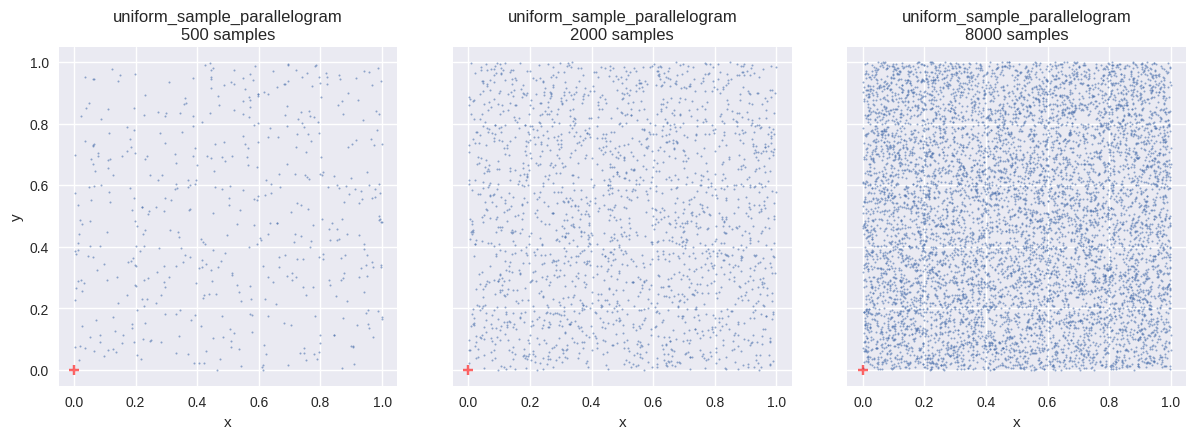
2.1 平行四辺形（parallelogram）内の一様分布

確率変数 \(\boldsymbol{X}\) が、平面上の領域 \(S\) 内に一様分布するとする．

\[ S: \boldsymbol{x}(u,v)=\boldsymbol{x}_{1}+u(\boldsymbol{x}_{2}-\boldsymbol{x}_{1})+v(\boldsymbol{x}_{4}-\boldsymbol{x}_{1}) ,\quad 0\le u,v\le 1 \]

\(\boldsymbol{x}_{i}\) は平行四辺形の頂点であり，辺の対応は，

\[ \boldsymbol{x}_{3} =\boldsymbol{x}_{2}+\boldsymbol{x}_{4}-\boldsymbol{x}_{1} \]

で定まるものとする．同時確率密度関数は領域 \(S\) で定数 \(c\) であり，正規化条件を考える．面積要素は，

\[ dS =\left\|\frac{\partial\boldsymbol{x}}{\partial u}\times\frac{\partial\boldsymbol{x}}{\partial v}\right\|\,dudv =A\,dudv \]

ここで，平行四辺形の面積を \(A=\left\|\frac{\partial\boldsymbol{x}}{\partial u}\times\frac{\partial\boldsymbol{x}}{\partial v}\right\|\) とした．したがって，

\[ 1 =\iint_{S} c\,dS =\int_{0}^{1}\int_{0}^{1} cA\,dudv =c\cdot A \]

同時確率密度関数は，

\[ p_{\boldsymbol{X}}(\boldsymbol{x}) =\frac{1}{A} ,\quad p_{U,V}(u,v) =p_{\boldsymbol{X}}(\boldsymbol{x})\frac{dS}{dudv} =1 \]

周辺確率密度関数は，

\[ p_{U}(u) =\int_{0}^{1} p_{U,V}(u,v)\,dv =1 ,\quad p_{V}(v) =\int_{0}^{1} p_{U,V}(u,v)\,du =1 \]

累積分布関数は，

\[ P_{U}(u) =\int_{0}^{u} p_{U}(t)\,dt =u ,\quad P_{V}(v) =\int_{0}^{v} p_{V}(t)\,dt =v \]

逆関数は，

\[ P^{-1}_{U}(\zeta_{1}) =\zeta_{1} ,\quad P^{-1}_{V}(\zeta_{2}) =\zeta_{2} \]

def uniform_sample_parallelogram(u0, u1):
    return np.stack((u0, u1), axis=-1)


fn = uniform_sample_parallelogram  # type: ignore
title = f"{fn.__name__}\n{{}} samples"
distr_infos = [{"fn": fn, "num_samples": n, "title": title.format(n)} for n in SAMPLE_SIZES]

plot_distributions_2d(distr_infos, nrows_ncols=(int(math.ceil(len(distr_infos) / 3)), 3))

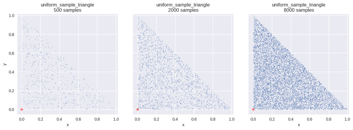
2.2 三角形（triangle）内の一様分布

確率変数 \(\boldsymbol{X}\) が、平面上の領域 \(S\) 内に一様分布するとする．

\[ S: \boldsymbol{x}(\lambda_{1},\lambda_{2})=\lambda_{1}\boldsymbol{x}_{1}+\lambda_{2}\boldsymbol{x}_{2}+(1-\lambda_{1}-\lambda_{2})\boldsymbol{x}_{3} ,\quad \lambda_{i}\ge 0,\,\lambda_{1}+\lambda_{2}\le 1 \]

同時確率密度関数は領域 \(S\) で定数 \(c\) であり，正規化条件を考える．面積要素は，

\[ dS =\left\|\frac{\partial\boldsymbol{x}}{\partial \lambda_{1}}\times\frac{\partial\boldsymbol{x}}{\partial \lambda_{2}}\right\|\,d\lambda_{1}d\lambda_{2} =2A\,d\lambda_{1}d\lambda_{2} \]

ここで，三角形の面積を \(A=\frac{1}{2}\left\|\frac{\partial\boldsymbol{x}}{\partial\lambda_{1}}\times\frac{\partial\boldsymbol{x}}{\partial\lambda_{2}}\right\|\) とした．したがって，

\[ 1 =\iint_{S} c\,dS =\int_{0}^{1}\int_{0}^{1-\lambda_{2}} c2A\,d\lambda_{1}d\lambda_{2} =c\cdot A \]

同時確率密度関数は，

\[ p_{\boldsymbol{X}}(\boldsymbol{x}) =\frac{1}{A} ,\quad p_{\Lambda_{1},\Lambda_{2}}(\lambda_{1},\lambda_{2}) =p_{\boldsymbol{X}}(\boldsymbol{x})\frac{dS}{d\lambda_{1}d\lambda_{2}} =2 \]

周辺確率密度関数は，

\[ p_{\Lambda_{1}}(\lambda_{1}) =\int_{0}^{1-\lambda_{1}} p_{\Lambda_{1},\Lambda_{2}}(\lambda_{1},\lambda_{2})\,d\lambda_{2} =2(1-\lambda_{1}) ,\quad p_{\Lambda_{2}}(\lambda_{2}) =\int_{0}^{1-\lambda_{2}} p_{\Lambda_{1},\Lambda_{2}}(\lambda_{1},\lambda_{2})\,d\lambda_{1} =2(1-\lambda_{2}) \]

\(\Lambda_{1}, \Lambda_{2}\) は独立ではないので，

\[ p_{\Lambda_{2}|\Lambda_{1}}(\lambda_{2}|\lambda_{1}) =\frac{p_{\Lambda_{1},\Lambda_{2}}(\lambda_{1},\lambda_{2})}{p_{\Lambda_{1}}(\lambda_{1})} =\frac{1}{1-\lambda_{1}} \]

累積分布関数は，

\[ P_{\Lambda_{1}}(\lambda_{1}) =\int_{0}^{\lambda_{1}} p_{\Lambda_{1}}(t)\,dt =2\lambda_{1}-\lambda^{2}_{1} ,\quad P_{\Lambda_{2}|\Lambda_{1}}(\lambda_{2}|\lambda_{1}) =\int_{0}^{\lambda_{2}} p_{\Lambda_{2}|\Lambda_{1}}(t|\lambda_{1})\,dt =\frac{\lambda_{2}}{1-\lambda_{1}} \]

逆関数は，

\[ P^{-1}_{\Lambda_{1}}(\zeta_{1}) =1-\sqrt{1-\zeta_{1}} ,\quad P^{-1}_{\Lambda_{2}|\Lambda_{1}}(\zeta_{2}|\lambda_{1}) =(1-\lambda_{1})\zeta_{2} \]

def uniform_sample_triangle(u0, u1):
    lambda0 = 1.0 - np.sqrt(u0)  # np.sqrt(1.0 - u0)
    lambda1 = (1.0 - lambda0) * u1
    x = (lambda0, lambda1)
    return np.stack(x, axis=-1)


fn = uniform_sample_triangle  # type: ignore
title = f"{fn.__name__}\n{{}} samples"
distr_infos = [{"fn": fn, "num_samples": n, "title": title.format(n)} for n in SAMPLE_SIZES]

plot_distributions_2d(distr_infos, nrows_ncols=(int(math.ceil(len(distr_infos) / 3)), 3))

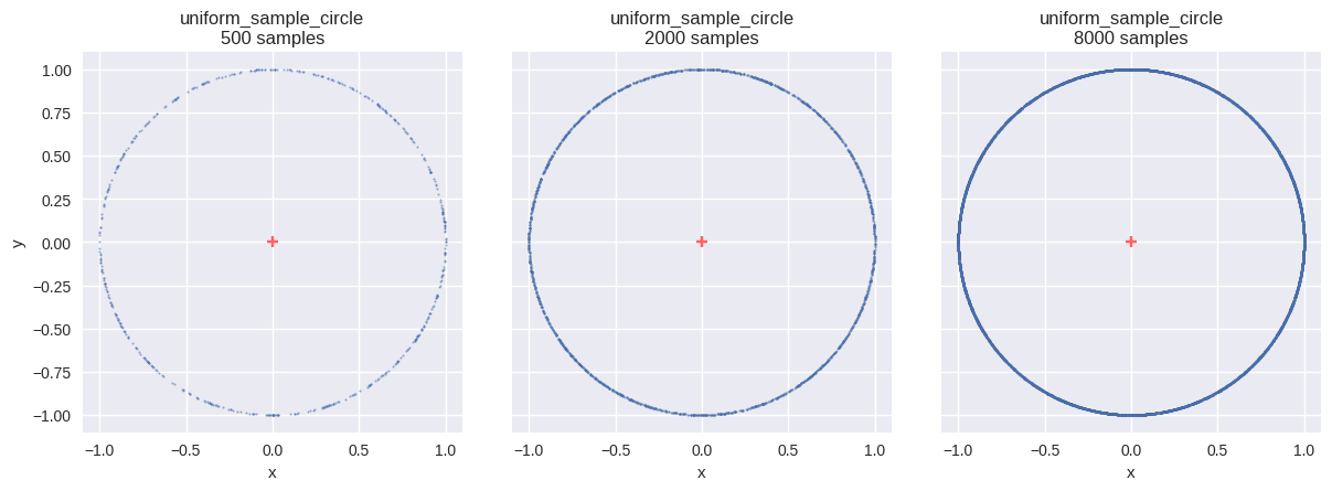
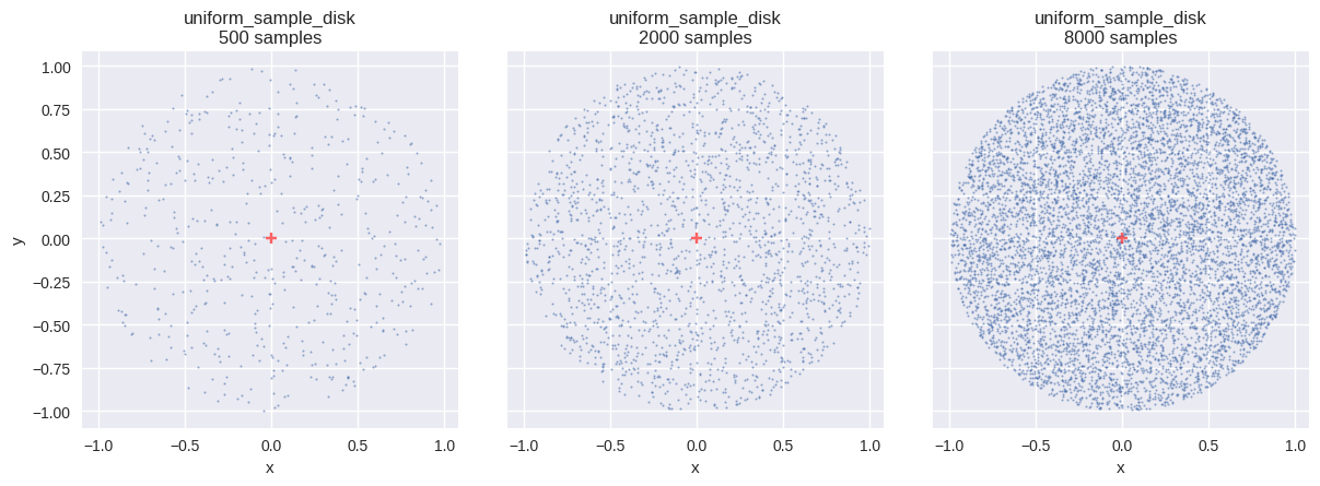
2.3 円板（disk）内の一様分布

確率変数 \(\boldsymbol{X}\) が、平面上の領域 \(S\) 内に一様分布するとする．

\[ S: \boldsymbol{x}(\rho,\phi)=\rho(\cos\phi\,\boldsymbol{b}_1+\sin\phi\,\boldsymbol{b}_2) ,\quad 0\le\rho\le R,\, 0\le\phi\lt 2\pi \]

同時確率密度関数は領域 \(S\) で定数 \(c\) であり，正規化条件を考える．面積要素は，

\[ dS =\left\|\frac{\partial\boldsymbol{x}}{\partial\rho}\times\frac{\partial\boldsymbol{x}}{\partial\phi}\right\|\,d\rho d\phi =\rho\,d\rho d\phi \]

したがって，

\[ 1 =\iint_{S} c\,dS =\int_{0}^{2\pi}\int_{0}^{R} c\rho\,d\rho d\phi =c\cdot \pi R^{2} \]

同時確率密度関数は，

\[ p_{\boldsymbol{X}}(\boldsymbol{x}) =\frac{1}{\pi R^{2}} ,\quad p_{\mathrm{P},\Phi}(\rho,\phi) =p_{\boldsymbol{X}}(\boldsymbol{x})\frac{dS}{d\rho d\phi} =\frac{\rho}{\pi R^{2}} \]

周辺確率密度関数は，

\[ p_{\mathrm{P}}(\rho) =\int_{0}^{2\pi} p_{\mathrm{P},\Phi}(\rho,\phi)\,d\phi =\frac{2\rho}{R^{2}} ,\quad p_{\Phi}(\phi) =\int_{0}^{R} p_{\mathrm{P},\Phi}(\rho,\phi)\,d\rho =\frac{1}{2\pi} \]

累積分布関数は，

\[ P_{\mathrm{P}}(\rho) =\int_{0}^{\rho} p_{\mathrm{P}}(t)\,dt =\frac{\rho^{2}}{R^{2}} ,\quad P_{\Phi}(\phi) =\int_{0}^{\phi} p_{\Phi}(t)\,dt =\frac{\phi}{2\pi} \]

逆関数は，

\[ P^{-1}_{\mathrm{P}}(\zeta_{1}) =R\sqrt{\zeta_{1}} ,\quad P^{-1}_{\Phi}(\zeta_{2}) =2\pi\zeta_{2} \]

def uniform_sample_disk(u0, u1):
    rho = np.sqrt(u0)
    phi = 2.0 * np.pi * u1
    x = (np.cos(phi), np.sin(phi))
    return rho[:, np.newaxis] * np.stack(x, axis=-1)


fn = uniform_sample_disk  # type: ignore
title = f"{fn.__name__}\n{{}} samples"
distr_infos = [{"fn": fn, "num_samples": n, "title": title.format(n)} for n in SAMPLE_SIZES]

plot_distributions_2d(distr_infos, nrows_ncols=(int(math.ceil(len(distr_infos) / 3)), 3))

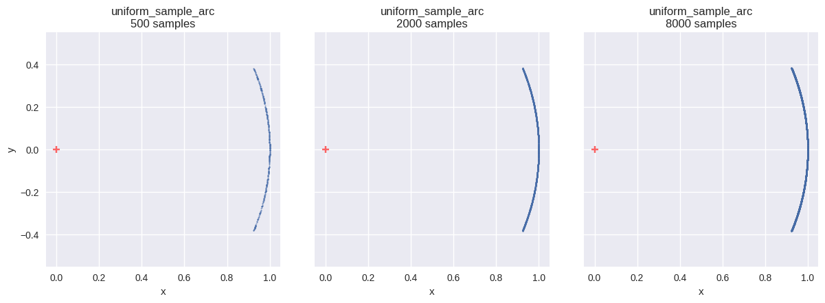
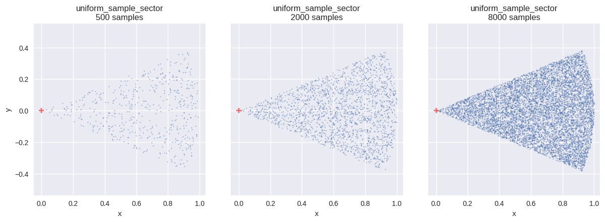
2.4 扇形（sector）内の一様分布

確率変数 \(\boldsymbol{X}\) が、平面上の領域 \(S\) 内に一様分布するとする．

\[ S: \boldsymbol{x}(\rho,\phi)=\rho(\cos\phi\,\boldsymbol{b}_1+\sin\phi\,\boldsymbol{b}_2) ,\quad 0\le\rho\le R,\, -\frac{\phi_{\text{max}}}{2}\le\phi\le\frac{\phi_{\text{max}}}{2} \]

同時確率密度関数は領域 \(S\) で定数 \(c\) であり，正規化条件を考える．面積要素は，

\[ dS =\left\|\frac{\partial\boldsymbol{x}}{\partial\rho}\times\frac{\partial\boldsymbol{x}}{\partial\phi}\right\|\,d\rho d\phi =\rho\,d\rho d\phi \]

したがって，

\[ 1 =\iint_{S} c\,dS =\int_{-\frac{\phi_{\text{max}}}{2}}^{\frac{\phi_{\text{max}}}{2}}\int_{0}^{R} c\rho\,d\rho d\phi =c\cdot \frac{R^{2}\phi_{\text{max}}}{2} \]

同時確率密度関数は，

\[ p_{\boldsymbol{X}}(\boldsymbol{x}) =\frac{2}{R^{2}\phi_{\text{max}}} ,\quad p_{\mathrm{P},\phi}(\rho,\phi) =p_{\boldsymbol{X}}(\boldsymbol{x})\frac{dS}{d\rho d\phi} =\frac{2\rho}{R^{2}\phi_{\text{max}}} \]

周辺確率密度関数は，

\[ p_{\mathrm{P}}(\rho) =\int_{-\frac{\phi_{\text{max}}}{2}}^{\frac{\phi_{\text{max}}}{2}} p_{\mathrm{P},\phi}(\rho,\phi)\,d\phi =\frac{2\rho}{R^{2}} ,\quad p_{\Phi}(\phi) =\int_{0}^{R} p_{\mathrm{P},\phi}(\rho,\phi)\,d\rho =\frac{1}{\phi_{\text{max}}} \]

累積分布関数は，

\[ P_{\mathrm{P}}(\rho) =\int_{0}^{\rho} p_{\mathrm{P}}(t)\,dt =\frac{\rho^{2}}{R^{2}} ,\quad P_{\Phi}(\phi) =\int_{-\frac{\phi_{\text{max}}}{2}}^{\phi} p_{\Phi}(t)\,dt =\frac{\phi+\frac{\phi_{\text{max}}}{2}}{\phi_{\text{max}}} \]

逆関数は，

\[ P^{-1}_{\mathrm{P}}(\zeta_{1}) =R\sqrt{\zeta_{1}} ,\quad P^{-1}_{\Phi}(\zeta_{2}) =\phi_{\text{max}}\left(\zeta_{2}-\frac{1}{2}\right) \]

def uniform_sample_sector(u0, u1, *, phi_max=np.pi):
    rho = np.sqrt(u0)
    phi = phi_max * (u1 - 0.5)
    x = (np.cos(phi), np.sin(phi))
    return rho[:, np.newaxis] * np.stack(x, axis=-1)


fn = uniform_sample_sector  # type: ignore
fn_kwargs = {"phi_max": 0.25 * np.pi}
title = f"{fn.__name__}\n{{}} samples"
distr_infos = [{"fn": fn, "num_samples": n, "fn_kwargs": fn_kwargs, "title": title.format(n)} for n in SAMPLE_SIZES]

plot_distributions_2d(distr_infos, nrows_ncols=(int(math.ceil(len(distr_infos) / 3)), 3))

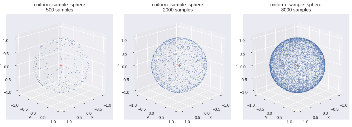
2.5 球（sphere）上の一様分布

確率変数 \(\boldsymbol{X}\) が，曲面 \(S\) 上に一様分布するとする．

\[ S: \boldsymbol{x}(\theta,\phi)= \begin{pmatrix} R\sin\theta\cos\phi\\ R\sin\theta\sin\phi\\ R\cos\theta \end{pmatrix} ,\quad 0\le\theta\le\pi,\,0\le\phi\lt 2\pi \]

同時確率密度関数は曲面 \(S\) で定数 \(c\) であり，正規化条件を考える．面積要素は，

\[ dS =\left\|\frac{\partial\boldsymbol{x}}{\partial\theta}\times\frac{\partial\boldsymbol{x}}{\partial\phi}\right\|\,d\theta d\phi =R^{2}\sin\theta\,d\theta d\phi \]

したがって，

\[ 1 =\int_{S} c\,dS =\int_{0}^{2\pi}\int_{0}^{\pi} cR^{2}\sin\theta\,d\theta d\phi =c\cdot 4\pi R^{2} \]

同時確率密度関数は，

\[ p_{\boldsymbol{X}}(\boldsymbol{x}) =\frac{1}{4\pi R^{2}} ,\quad p_{\Theta,\Phi}(\theta,\phi) =p_{\boldsymbol{X}}(\boldsymbol{x})\frac{dS}{d\theta d\phi} =\frac{\sin\theta}{4\pi} \]

周辺確率密度関数は，

\[ p_{\Theta}(\theta) =\int_{0}^{2\pi} p_{\Theta,\Phi}(\theta,\phi)\,d\phi =\frac{\sin\theta}{2} ,\quad p_{\Phi}(\phi) =\int_{0}^{\pi} p_{\Theta,\Phi}(\theta,\phi)\,d\theta =\frac{1}{2\pi} \]

累積分布関数は，

\[ P_{\Theta}(\theta) =\int_{0}^{\theta} p_{\Theta}(t)\,dt =\frac{1-\cos\theta}{2} ,\quad P_{\Phi}(\phi) =\int_{0}^{\phi} p_{\Phi}(t)\,dt =\frac{\phi}{2\pi} \]

逆関数は，

\[ P^{-1}_{\Theta}(\zeta_{1}) =\arccos(1-2\zeta_{1}) ,\quad P^{-1}_{\Phi}(\zeta_{2}) =2\pi\zeta_{2} \]

def uniform_sample_sphere(u0, u1):
    c = 1.0 - 2.0 * u0
    s = np.sqrt(1.0 - c * c)
    phi = 2.0 * np.pi * u1
    w = (s * np.cos(phi), s * np.sin(phi), c)
    return np.stack(w, axis=-1)


fn = uniform_sample_sphere  # type: ignore
title = f"{fn.__name__}\n{{}} samples"
distr_infos = [{"fn": fn, "num_samples": n, "title": title.format(n)} for n in SAMPLE_SIZES]

plot_distributions_3d(distr_infos, nrows_ncols=(int(math.ceil(len(distr_infos) / 3)), 3))

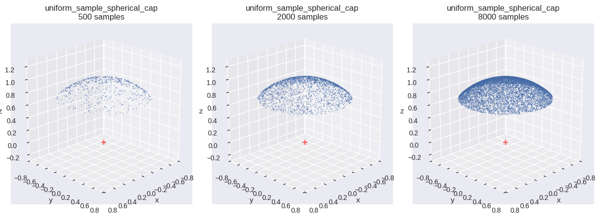
2.6 球冠（spherical cap）上の一様分布

確率変数 \(\boldsymbol{X}\) が，曲面 \(S\) 上で一様分布するとする．

\[ S: \boldsymbol{x}(\theta,\phi)= \begin{pmatrix} R\sin\theta\cos\phi\\ R\sin\theta\sin\phi\\ R\cos\theta \end{pmatrix} ,\quad 0\le\theta\le\theta_{\text{max}},\,0\le\phi\lt 2\pi \]

同時確率密度関数は曲面 \(S\) で定数 \(c\) であり，正規化条件を考える．面積要素は，

\[ dS =\left\|\frac{\partial\boldsymbol{x}}{\partial\theta}\times\frac{\partial\boldsymbol{x}}{\partial\phi}\right\|\,d\theta d\phi =R^{2}\sin\theta\,d\theta d\phi \]

したがって，

\[ 1 =\int_{S} c\,dS =\int_{0}^{2\pi}\int_{0}^{\theta_{\text{max}}} cR^{2}\sin\theta\,d\theta d\phi =c\cdot 2\pi R^{2}(1-\cos\theta_{\text{max}}) \]

同時確率密度関数は，

\[ p_{\boldsymbol{X}}(\boldsymbol{x}) =\frac{1}{2\pi R^{2}(1-\cos\theta_{\text{max}})} ,\quad p_{\Theta,\Phi}(\theta,\phi) =p_{\boldsymbol{X}}(\boldsymbol{x})\frac{dS}{d\theta d\phi} =\frac{\sin\theta}{2\pi(1-\cos\theta_{\text{max}})} \]

周辺確率密度関数は，

\[ p_{\Theta}(\theta) =\int_{0}^{2\pi} p_{\Theta,\Phi}(\theta,\phi)\,d\phi =\frac{\sin\theta}{1-\cos\theta_{\text{max}}} ,\quad p_{\Phi}(\phi) =\int_{0}^{\theta_{\text{max}}} p_{\Theta,\Phi}(\theta,\phi)\,d\theta =\frac{1}{2\pi} \]

累積分布関数は，

\[ P_{\Theta}(\theta) =\int_{0}^{\theta} p_{\Theta}(t)\,dt =\frac{1-\cos\theta}{1-\cos\theta_{\text{max}}} ,\quad P_{\Phi}(\phi) =\int_{0}^{\phi} p_{\Phi}(t)\,dt =\frac{\phi}{2\pi} \]

逆関数は，

\[ P^{-1}_{\Theta}(\zeta_{1}) =\arccos(1-(1-\cos\theta_{\text{max}})\zeta_{1}) ,\quad P^{-1}_{\Phi}(\zeta_{2}) =2\pi\zeta_{2} \]

def uniform_sample_spherical_cap(u0, u1, *, cos_theta_max=np.pi):
    c = 1.0 - (1.0 - cos_theta_max) * u0
    s = np.sqrt(1.0 - c * c)
    phi = 2.0 * np.pi * u1
    w = (s * np.cos(phi), s * np.sin(phi), c)
    return np.stack(w, axis=-1)


fn = uniform_sample_spherical_cap  # type: ignore
fn_kwargs = {"cos_theta_max": np.cos(0.25 * np.pi)}
title = f"{fn.__name__}\n{{}} samples"
distr_infos = [{"fn": fn, "num_samples": n, "fn_kwargs": fn_kwargs, "title": title.format(n)} for n in SAMPLE_SIZES]

plot_distributions_3d(distr_infos, nrows_ncols=(int(math.ceil(len(distr_infos) / 3)), 3))

2.7 単位半球（unit hemisphere）上の分布

確率変数 \(\boldsymbol{\Omega}\) が，単位半球上に分布するとする．

\[ H^{2}: \boldsymbol{\omega}(\theta, \phi)= \begin{pmatrix} \sin\theta\cos\phi\\ \sin\theta\sin\phi\\ \cos\theta \end{pmatrix} ,\quad 0\le\theta\le \frac{\pi}{2},\,0\le\phi\lt 2\pi \]

球面上の面積要素は，

\[ dA =\left\|\frac{\partial\boldsymbol{\omega}}{\partial\theta}\times\frac{\partial\boldsymbol{\omega}}{\partial\phi}\right\|\,d\theta d\phi =\sin\theta\,d\theta d\phi \]

であり，半径 \(r=1\) の単位球で立体角要素は，

\[ d\omega=\frac{dA}{r^{2}}=dA=\sin\theta\,d\theta d\phi \]

したがって，立体角上で定義された確率密度関数 \(p_{\boldsymbol{\Omega}}(\boldsymbol{\omega})\) は，測度変換により極座標系での同時確率密度関数 \(p_{\Theta,\Phi}(\theta,\phi)\) に次のように変換される．

\[ p_{\Theta,\Phi}(\theta,\phi) =p_{\boldsymbol{\Omega}}(\boldsymbol{\omega})\frac{d\omega}{d\theta d\phi} =p_{\boldsymbol{\Omega}}(\boldsymbol{\omega})\sin\theta \]

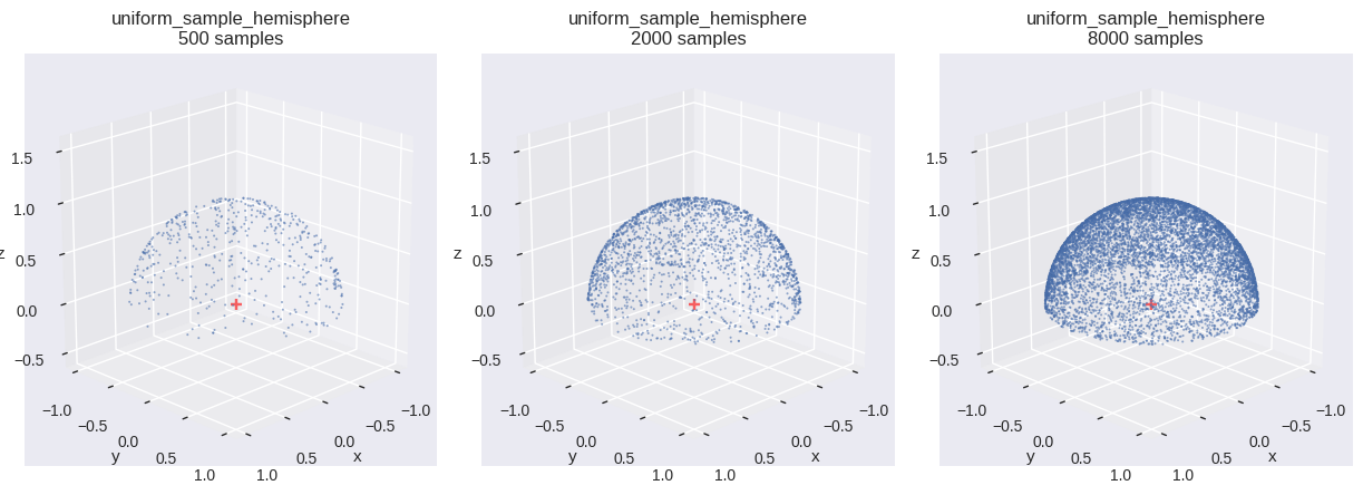
2.7.1 一様分布

確率変数 \(\boldsymbol{\Omega}\) が，単位半球上に一様分布するとする．このとき，同時確率密度関数は定数 \(c\) であり，正規化条件を考える．

\[ 1 =\int_{H^{2}} c\,d\omega =\int_{0}^{2\pi}\int_{0}^{\frac{\pi}{2}} c\sin\theta\,d\theta d\phi =c\cdot 2\pi \]

同時確率密度関数は，

\[ p_{\boldsymbol{\Omega}}(\boldsymbol{\omega}) =\frac{1}{2\pi} ,\quad p_{\Theta,\Phi}(\theta,\phi) =\frac{\sin\theta}{2\pi} \]

周辺確率密度関数は，

\[ p_{\Theta}(\theta) =\int_{0}^{2\pi} p_{\Theta,\Phi}(\theta,\phi)\,d\phi =\sin\theta ,\quad p_{\Phi}(\phi) =\int_{0}^{\frac{\pi}{2}} p_{\Theta,\Phi}(\theta,\phi)\,d\theta =\frac{1}{2\pi} \]

累積分布関数は，

\[ P_{\Theta}(\theta) =\int_{0}^{\theta} p_{\Theta}(t)\,dt =1-\cos\theta ,\quad P_{\Phi}(\phi) =\int_{0}^{\phi} p_{\Phi}(t)\,dt =\frac{\phi}{2\pi} \]

逆関数は，

\[ P^{-1}_{\Theta}(\zeta_{1}) =\arccos(1-\zeta_{1}) ,\quad P^{-1}_{\Phi}(\zeta_{2}) =2\pi\zeta_{2} \]

def uniform_sample_hemisphere(u0, u1):
    c = u0  # 1 - u0
    s = np.sqrt(1.0 - c * c)
    phi = 2.0 * np.pi * u1
    w = (s * np.cos(phi), s * np.sin(phi), c)
    return np.stack(w, axis=-1)


fn = uniform_sample_hemisphere  # type: ignore
title = f"{fn.__name__}\n{{}} samples"
distr_infos = [{"fn": fn, "num_samples": n, "title": title.format(n)} for n in SAMPLE_SIZES]

plot_distributions_3d(distr_infos, nrows_ncols=(int(math.ceil(len(distr_infos) / 3)), 3))

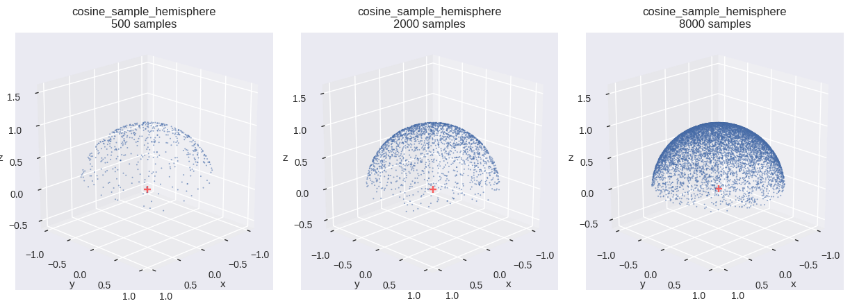
2.7.2 コサイン重み付き分布

確率変数 \(\boldsymbol{\Omega}\) が，単位半球上に \(\cos\theta\) に比例分布するとする．このとき，同時確率密度関数は \(c\cos\theta\) であり，正規化条件を考える．

\[ 1 =\int_{H^{2}} c\cos\theta\,d\omega =\int_{0}^{2\pi}\int_{0}^{\frac{\pi}{2}} c\cos\theta\sin\theta\,d\theta d\phi =c\cdot 2\pi\int_{0}^{1} u\,du =c\cdot\pi \]

同時確率密度関数は，

\[ p_{\boldsymbol{\Omega}}(\boldsymbol{\omega}) =\frac{\cos\theta}{\pi} ,\quad p_{\Theta,\Phi}(\theta,\phi) =\frac{\sin 2\theta}{2\pi} \]

周辺確率密度関数は，

\[ p_{\Theta}(\theta) =\int_{0}^{2\pi} p_{\Theta,\Phi}(\theta,\phi)\,d\phi =\sin 2\theta ,\quad p_{\Phi}(\phi) =\int_{0}^{\frac{\pi}{2}} p_{\Theta,\Phi}(\theta,\phi)\,d\theta =\frac{1}{2\pi} \]

累積分布関数は，

\[ P_{\Theta}(\theta) =\int_{0}^{\theta} p_{\Theta}(t)\,dt =\frac{1-\cos 2\theta}{2} =\sin^{2}\theta ,\quad P_{\Phi}(\phi) =\int_{0}^{\phi} p_{\Phi}(t)\,dt =\frac{\phi}{2\pi} \]

逆関数は，

\[ P^{-1}_{\Theta}(\zeta_{1}) =\arcsin\sqrt{\zeta_{1}} ,\quad P^{-1}_{\Phi}(\zeta_{2}) =2\pi\zeta_{2} \]

def cosine_sample_hemisphere(u0, u1):
    s = np.sqrt(u0)
    phi = 2.0 * np.pi * u1
    w = (s * np.cos(phi), s * np.sin(phi), np.sqrt(1.0 - u0))  # since u0 represents sin^2(theta)
    return np.stack(w, axis=-1)


fn = cosine_sample_hemisphere  # type: ignore
title = f"{fn.__name__}\n{{}} samples"
distr_infos = [{"fn": fn, "num_samples": n, "title": title.format(n)} for n in SAMPLE_SIZES]

plot_distributions_3d(distr_infos, nrows_ncols=(int(math.ceil(len(distr_infos) / 3)), 3))

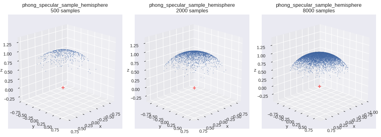
2.7.3 Phong Specular Lobe 分布

確率変数 \(\boldsymbol{\Omega}\) が，単位半球上に \(\cos^{n}\theta\) に比例分布するとする．このとき，同時確率密度関数は \(c\cos^{n}\theta\) であり，正規化条件を考える．

\[ 1 =\int_{H^{2}} c\cos^{n}\theta\,d\omega =\int_{0}^{2\pi}\int_{0}^{\frac{\pi}{2}} c\cos^{n}\theta\sin\theta\,d\theta d\phi =c\cdot 2\pi\int_{0}^{1} u^{n}\,du =c\cdot \frac{2\pi}{n+1} \]

同時確率密度関数は，

\[ p_{\boldsymbol{\Omega}}(\boldsymbol{\omega}) =\frac{n+1}{2\pi}\cos^{n}\theta ,\quad p_{\Theta,\Phi}(\theta,\phi) =\frac{n+1}{2\pi}\cos^{n}\theta\sin\theta \]

周辺確率密度関数は，

\[ p_{\Theta}(\theta) =\int_{0}^{2\pi} p_{\Theta,\Phi}(\theta,\phi)\,d\phi =(n+1)\cos^{n}\theta\sin\theta ,\quad p_{\Phi}(\phi) =\int_{0}^{\frac{\pi}{2}} p_{\Theta,\Phi}(\theta,\phi)\,d\theta =\frac{1}{2\pi} \]

累積分布関数は，

\[ P_{\Theta}(\theta) =\int_{0}^{\theta} p_{\Theta}(t)\,dt =1-\cos^{n+1}\theta ,\quad P_{\Phi}(\phi) =\int_{0}^{\phi} p_{\Phi}(t)\,dt =\frac{\phi}{2\pi} \]

逆関数は，

\[ P^{-1}_{\Theta}(\zeta_{1}) =\arccos\sqrt[n+1]{1-\zeta_{1}} \hspace{0.5em},\quad P^{-1}_{\Phi}(\zeta_{2}) =2\pi\zeta_{2} \]

def phong_specular_sample_hemisphere(u0, u1, *, n=2):
    c = (1.0 - u0) ** (1.0 / (n + 1))
    s = np.sqrt(1.0 - c * c)
    phi = 2.0 * np.pi * u1
    w = (s * np.cos(phi), s * np.sin(phi), c)
    return np.stack(w, axis=-1)


fn = phong_specular_sample_hemisphere  # type: ignore
fn_kwargs = {"n": 10}
title = f"{fn.__name__}\n{{}} samples"
distr_infos = [{"fn": fn, "num_samples": n, "fn_kwargs": fn_kwargs, "title": title.format(n)} for n in SAMPLE_SIZES]

plot_distributions_3d(distr_infos, nrows_ncols=(int(math.ceil(len(distr_infos) / 3)), 3))

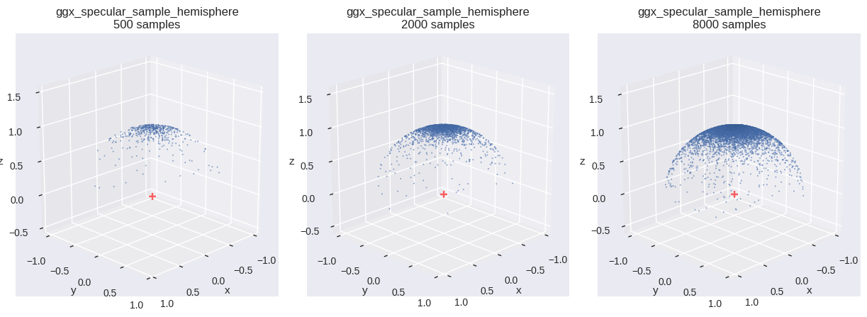
2.7.4 Microfacet GGX Specular Lobe 分布

確率変数 \(\boldsymbol{\Omega}\) が，単位半球上に \(D(\theta)\cos\theta\) に比例分布するとする．ここで GGX の NDF を，

\[ D(\theta) =\frac{\alpha^{2}}{\pi\left(\cos^{2}\theta\,(\alpha^{2}-1)+1\right)^{2}} \]

と定める．同時確率密度関数は \(cD(\theta)\cos\theta\) であり，正規化条件を考える．

\[ \begin{align*} 1 &=\int_{H^{2}} cD(\theta)\cos\theta\,d\omega =\int_{0}^{2\pi}\int_{0}^{\frac{\pi}{2}} cD(\theta)\cos\theta\sin\theta\,d\theta d\phi\\ &=c\cdot\alpha^{2}\int_{0}^{1}\frac{1}{\left(u(\alpha^{2}-1)+1 \right)^{2}}\,du \quad(u=\cos^{2}\theta)\\ &=c\cdot\frac{\alpha^{2}}{\alpha^{2}-1}\int_{1}^{\alpha^{2}}\frac{1}{v^{2}}\,dv \quad(v=u(\alpha^{2}-1)+1)\\ &=c \end{align*} \]

同時確率密度関数は，

\[ p_{\boldsymbol{\Omega}}(\boldsymbol{\omega}) =D(\theta)\cos\theta ,\quad p_{\Theta,\Phi}(\theta,\phi) =D(\theta)\cos\theta\sin\theta \]

周辺確率密度関数は，

\[ p_{\Theta}(\theta) =\int_{0}^{2\pi} p_{\Theta,\Phi}(\theta,\phi)\,d\phi =2\pi D(\theta)\cos\theta\sin\theta ,\quad p_{\Phi}(\phi) =\int_{0}^{\frac{\pi}{2}} p_{\Theta,\Phi}(\theta,\phi)\,d\theta =\frac{1}{2\pi} \]

累積分布関数は，

\[ P_{\Theta}(\theta) =\int_{0}^{\theta} p_{\Theta}(t)\,dt =\frac{1-\cos^{2}\theta}{\cos^{2}\theta\,(\alpha^{2}-1)+1} ,\quad P_{\Phi}(\phi) =\int_{0}^{\phi} p_{\Phi}(t)\,dt =\frac{\phi}{2\pi} \]

逆関数は，

\[ P^{-1}_{\Theta}(\zeta_{1}) =\arccos\sqrt{\frac{1-\zeta_{1}}{(\alpha^{2}-1)\zeta_{1}+1}} ,\quad P^{-1}_{\Phi}(\zeta_{2}) =2\pi\zeta_{2} \]

def ggx_specular_sample_hemisphere(u0, u1, *, alpha=1.0):
    c = np.sqrt((1.0 - u0) / ((alpha * alpha - 1.0) * u0 + 1.0))
    s = np.sqrt(1.0 - c * c)
    phi = 2.0 * np.pi * u1
    w = (s * np.cos(phi), s * np.sin(phi), c)
    return np.stack(w, axis=-1)


fn = ggx_specular_sample_hemisphere  # type: ignore
roughness = 0.5
fn_kwargs = {"alpha": roughness**2.0}
title = f"{fn.__name__}\n{{}} samples"
distr_infos = [{"fn": fn, "num_samples": n, "fn_kwargs": fn_kwargs, "title": title.format(n)} for n in SAMPLE_SIZES]

plot_distributions_3d(distr_infos, nrows_ncols=(int(math.ceil(len(distr_infos) / 3)), 3))

3 ３次元サンプリング

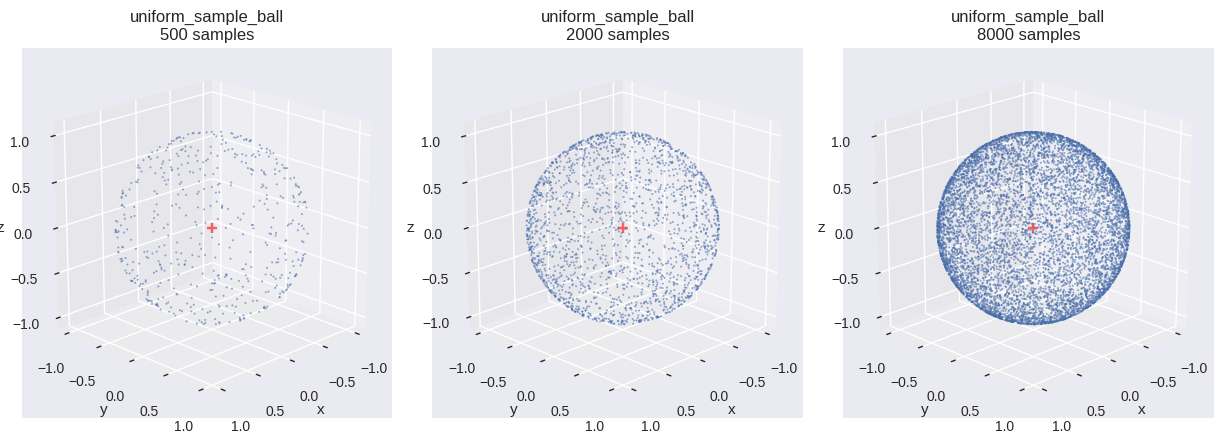
3.1 球体（ball）内の一様分布

確率変数 \(\boldsymbol{X}\) が領域 \(V\) 内に一様分布するとする．

\[ V: \boldsymbol{x}(r,\theta,\phi)= \begin{pmatrix} r\sin\theta\cos\phi\\ r\sin\theta\sin\phi\\ r\cos\theta \end{pmatrix} ,\quad 0\le r\le R,\,0\le\theta\le\pi,\,0\le\phi\lt 2\pi \]

同時確率密度関数は領域 \(V\) で定数 \(c\) であり，正規化条件を考える．体積要素は，

\[ dV =\left|\frac{\partial(x,y,z)}{\partial(r,\theta,\phi)}\right|\,drd\theta d\phi =r^{2}\sin\theta\,drd\theta d\phi \]

したがって，

\[ 1 =\int_{V} c\,dV =\int_{0}^{2\pi}\int_{0}^{\pi}\int_{0}^{R} cr^{2}\sin\theta\,drd\theta d\phi =c\cdot\frac{4\pi R^{3}}{3} \]

同時確率密度関数は，

\[ p_{\boldsymbol{X}}(\boldsymbol{x}) =\frac{3}{4\pi R^{3}} ,\quad p_{R,\Theta,\Phi}(r,\theta,\phi) =p_{\boldsymbol{X}}(\boldsymbol{x})\frac{dV}{drd\theta d\phi} =\frac{3}{4\pi R^{3}}r^{2}\sin\theta \]

周辺確率密度関数は，

\[ \begin{align*} p_{R}(r) &=\int_{0}^{2\pi}\int_{0}^{\pi} p_{R,\Theta,\Phi}(r,\theta,\phi)\,d\theta d\phi =\frac{3r^{2}}{R^{3}}\\ p_{\Theta}(\theta) &=\int_{0}^{2\pi}\int_{0}^{R} p_{R,\Theta,\Phi}(r,\theta,\phi)\,drd\phi =\frac{\sin\theta}{2}\\ p_{\Phi}(\phi) &=\int_{0}^{\pi}\int_{0}^{R} p_{R,\Theta,\Phi}(r,\theta,\phi)\,drd\theta =\frac{1}{2\pi} \end{align*} \]

累積分布関数は，

\[ P_{R}(r) =\int_{0}^{r} p_{R}(t)\,dt =\frac{r^{3}}{R^{3}} ,\quad P_{\Theta}(\theta) =\int_{0}^{\theta} p_{\Theta}(t)\,dt =\frac{1-\cos\theta}{2} ,\quad P_{\Phi}(\phi) =\int_{0}^{\phi} p_{\Phi}(t)\,dt =\frac{\phi}{2\pi} \]

逆関数は，

\[ P^{-1}_{R}(\zeta_{1}) =R\sqrt[3]{\zeta_{1}} ,\quad P^{-1}_{\Theta}(\zeta_{2}) =\arccos(1-2\zeta_{2}) ,\quad P^{-1}_{\Phi}(\zeta_{3}) =2\pi\zeta_{3} \]

def uniform_sample_ball(u0, u1, u2):
    radius = np.cbrt(u0)
    c = 1.0 - 2.0 * u1
    s = np.sqrt(1.0 - c * c)
    phi = 2.0 * np.pi * u2
    w = (s * np.cos(phi), s * np.sin(phi), c)
    return np.stack(w, axis=-1)


fn = uniform_sample_ball  # type: ignore
title = f"{fn.__name__}\n{{}} samples"
distr_infos = [{"fn": fn, "num_samples": n, "title": title.format(n)} for n in SAMPLE_SIZES]

plot_distributions_3d(distr_infos, nrows_ncols=(int(math.ceil(len(distr_infos) / 3)), 3))

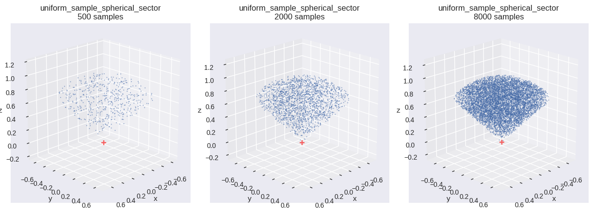
3.2 球扇形（spherical sector）内の一様分布

確率変数 \(\boldsymbol{X}\) が領域 \(V\) 内に一様分布するとする．

\[ V: \boldsymbol{x}(r,\theta,\phi)= \begin{pmatrix} r\sin\theta\cos\phi\\ r\sin\theta\sin\phi\\ r\cos\theta \end{pmatrix} ,\quad 0\le r\le R,\,0\le\theta\le\theta_{\text{max}},\,0\le\phi\lt 2\pi \]

同時確率密度関数は領域 \(V\) で定数 \(c\) であり，正規化条件を考える．体積要素は，

\[ dV =\left|\frac{\partial(x,y,z)}{\partial(r,\theta,\phi)}\right|\,drd\theta d\phi =r^{2}\sin\theta\,drd\theta d\phi \]

したがって，

\[ 1 =\int_{V} c\,dV =\int_{0}^{2\pi}\int_{0}^{\theta_{\text{max}}}\int_{0}^{R} cr^{2}\sin\theta\,drd\theta d\phi =c\cdot\frac{2\pi R^{3}}{3}(1-\cos\theta_{\text{max}}) \]

同時確率密度関数は，

\[ p_{\boldsymbol{X}}(\boldsymbol{x}) =\frac{3}{2\pi R^{3}(1-\cos\theta_{\text{max}})} ,\quad p_{R,\Theta,\Phi}(r,\theta,\phi) =p_{\boldsymbol{X}}(\boldsymbol{x})\frac{dV}{drd\theta d\phi} =\frac{3r^{2}\sin\theta}{2\pi R^{3}(1-\cos\theta_{\text{max}})} \]

周辺確率密度関数は，

\[ \begin{align*} p_{R}(r) &=\int_{0}^{2\pi}\int_{0}^{\theta_{\text{max}}} p_{R,\Theta,\Phi}(r,\theta,\phi)\,d\theta d\phi =\frac{3r^{2}}{R^{3}}\\ p_{\Theta}(\theta) &=\int_{0}^{2\pi}\int_{0}^{R} p_{R,\Theta,\Phi}(r,\theta,\phi)\,drd\phi =\frac{\sin\theta}{1-\cos\theta_{\text{max}}}\\ p_{\Phi}(\phi) &=\int_{0}^{\theta_{\text{max}}}\int_{0}^{R} p_{R,\Theta,\Phi}(r,\theta,\phi)\,drd\theta =\frac{1}{2\pi} \end{align*} \]

累積分布関数は，

\[ P_{R}(r) =\int_{0}^{r} p_{R}(t)\,dt =\frac{r^{3}}{R^{3}} ,\quad P_{\Theta}(\theta) =\int_{0}^{\theta} p_{\Theta}(t)\,dt =\frac{1-\cos\theta}{1-\cos\theta_{\text{max}}} ,\quad P_{\Phi}(\phi) =\int_{0}^{\phi} p_{\Phi}(t)\,dt =\frac{\phi}{2\pi} \]

逆関数は，

\[ P^{-1}_{R}(\zeta_{1}) =R\sqrt[3]{\zeta_{1}} ,\quad P^{-1}_{\Theta}(\zeta_{2}) =\arccos(1-(1-\cos\theta_{\text{max}})\zeta_{2}) ,\quad P^{-1}_{\Phi}(\zeta_{3}) =2\pi\zeta_{3} \]

def uniform_sample_spherical_sector(u0, u1, u2, *, cos_theta_max=np.pi):
    radius = np.cbrt(u0)
    c = 1.0 - (1.0 - cos_theta_max) * u1
    s = np.sqrt(1.0 - c * c)
    phi = 2.0 * np.pi * u2
    w = (s * np.cos(phi), s * np.sin(phi), c)
    return radius[:, np.newaxis] * np.stack(w, axis=-1)


fn = uniform_sample_spherical_sector  # type: ignore
fn_kwargs = {"cos_theta_max": np.cos(0.25 * np.pi)}
title = f"{fn.__name__}\n{{}} samples"
distr_infos = [{"fn": fn, "num_samples": n, "fn_kwargs": fn_kwargs, "title": title.format(n)} for n in SAMPLE_SIZES]

plot_distributions_3d(distr_infos, nrows_ncols=(int(math.ceil(len(distr_infos) / 3)), 3))

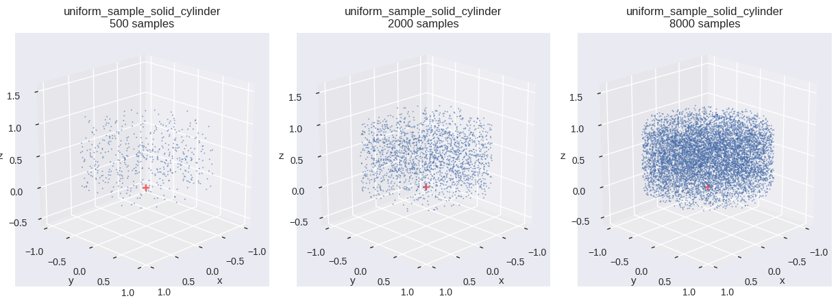
3.3 円柱（solid cylinder）内の一様分布

確率変数 \(\boldsymbol{X}\) が領域 \(V\) 内に一様分布するとする．

\[ V: \boldsymbol{x}(\rho,\phi,z)= \begin{pmatrix} \rho\cos\phi\\ \rho\sin\phi\\ z \end{pmatrix} ,\quad 0\le\rho\le R,\,0\le\phi\lt 2\pi,\,0\le z\le H \]

同時確率密度関数は領域 \(V\) で定数 \(c\) であり，正規化条件を考える．体積要素は，

\[ dV =\left|\frac{\partial(x,y,z)}{\partial(\rho,\phi,z)}\right|\,d\rho d\phi dz =\rho\,d\rho d\phi dz \]

したがって，

\[ 1 =\int_{V} c\,dV =\int_{0}^{H}\int_{0}^{2\pi}\int_{0}^{R} c\rho\,d\rho d\phi dz =c\cdot \pi R^{2}H \]

同時確率密度関数は，

\[ p_{\boldsymbol{X}}(\boldsymbol{x}) =\frac{1}{\pi R^{2}H} ,\quad p_{\mathrm{P},\Phi,Z}(\rho,\phi,z) =p_{\boldsymbol{X}}(\boldsymbol{x})\frac{dV}{d\rho d\phi dz} =\frac{\rho}{\pi R^{2}H} \]

周辺確率密度関数は，

\[ \begin{align*} p_{\mathrm{P}}(\rho) &=\int_{0}^{H}\int_{0}^{2\pi} p_{\mathrm{P},\Phi,Z}(\rho,\phi,z)\,d\phi dz =\frac{2\rho}{R^{2}}\\ p_{\Phi}(\phi) &=\int_{0}^{H}\int_{0}^{R} p_{\mathrm{P},\Phi,Z}(\rho,\phi,z)\,d\rho dz =\frac{1}{2\pi}\\ p_{Z}(z) &=\int_{0}^{2\pi}\int_{0}^{R} p_{\mathrm{P},\Phi,Z}(\rho,\phi,z)\,d\rho d\phi =\frac{1}{H} \end{align*} \]

累積分布関数は，

\[ P_{\mathrm{P}}(\rho) =\int_{0}^{\rho} p_{\mathrm{P}}(t)\,dt =\frac{\rho^{2}}{R^{2}} ,\quad P_{\Phi}(\phi) =\int_{0}^{\phi} p_{\Phi}(t)\,dt =\frac{\phi}{2\pi} ,\quad P_{Z}(z) =\int_{0}^{z} p_{Z}(t)\,dt =\frac{z}{H} \]

逆関数は，

\[ P^{-1}_{\mathrm{P}}(\zeta_{1}) =R\sqrt{\zeta_{1}} ,\quad P^{-1}_{\Phi}(\zeta_{2}) =2\pi\zeta_{2} ,\quad P^{-1}_{Z}(\zeta_{3}) =H\zeta_{3} \]

def uniform_sample_solid_cylinder(u0, u1, u2):
    rho = np.sqrt(u0)
    phi = 2.0 * np.pi * u1
    w = (rho * np.cos(phi), rho * np.sin(phi), u2)
    return np.stack(w, axis=-1)


fn = uniform_sample_solid_cylinder  # type: ignore
title = f"{fn.__name__}\n{{}} samples"
distr_infos = [{"fn": fn, "num_samples": n, "title": title.format(n)} for n in SAMPLE_SIZES]

plot_distributions_3d(distr_infos, nrows_ncols=(int(math.ceil(len(distr_infos) / 3)), 3))

4 References

• Pharr, M., Jakob, W., & Humphreys, G. (n.d.). 2D sampling with multidimensional transformations. Physically Based Rendering: From Theory To Implementation. https://www.pbr-book.org/3ed-2018/Monte_Carlo_Integration/2D_Sampling_with_Multidimensional_Transformations
• Kerbl, B. (n.d.). Rendering: Importance sampling. Research Division of Computer Graphics, Institute of Visual Computing & Human-Centered Technology, TU Wien, Austria. https://www.cg.tuwien.ac.at/sites/default/files/course/4411/attachments/06_importance_sampling_0.pdf
• Walter, B. (2005, April 29). Notes on the ward BRDF. Cornell Program of Computer Graphics. https://www.graphics.cornell.edu/~bjw/wardnotes.pdf
• Inverse transform sampling. (2025, August 26). In Wikipedia. https://en.wikipedia.org/w/index.php?title=Inverse_transform_sampling&oldid=1307944637